Introduction

Most programmers are familiar with code written as functions that take arguments that subsequently call more functions that take more arguments. In order to call a function you need to know what arguments to provide, and in addition that function needs to know what arguments to provide to functions it calls and possibly add them to its own argument list to be passed in.

MDF turns this around and provides a way of expressing code as a directed acylical graph, or DAG for short. Each node in the graph depends on other nodes, which ultimately may depend on a set of terminal nodes that represent the input values to the graph or sub-graph.

This is best explained via a brief example. Consider this set of simple Python functions:

def A(x, y, z):
    return B(x, y) + C(y, z)

def B(x, y):
    return x + y

def C(y, z):
    return y * z

This can be expressed as the following graph:

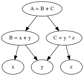
In the first case evaluating A(1, 2, 3) is simply a case of calling the function. In the second case, we evaluate the node A under the condition x=1, y=2 and z=3.

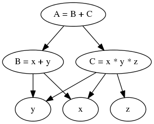
Consider that now the definiation of C is not quite right, it’s decided it should actually be:

def C(x, y, z):
    return x * y * z

Because of this change to C, now A has to changed. If it has required another argument then A would also have to have its arguments changed and and functions calling A would have to be updated:

def A(x, y, z):
    return B(x, y) + C(x, y, z)

def B(x, y):
    return x + y

def C(x, y, z):
    return x * y * z

In the graph based approach node C can be changed without impact on A, and provided all dependents of C exist in the graph there is no change required to the calling code.

Now consider that you want to evaluate A for a set of z. Using the traditional approach you could call A(x, y, z) for each z in the required set. Now assume that you also want to collect the values of C for that set of z as well as A. At this point you have a few choices. You might call A and C for each z, you might refactor A to take C as an argument so you only have to compute C once for each z, or you might refactor A to take a list as an argument and accumulate the results of C in that.

Let’s assume you end up with something like this:

def A(x, y, c):
    return B(x, y) + c

def B(x, y):
    return x + y

def C(x, y, z):
    return x * y * z

x = 1
y = 2
for z in range(100):
    c = C(x, y, z)
    a = A(a, y, c)
    print a, c

Now you notice that computing B every time is expensive and unnecessary. You refactor out B to improve performance:

def A(b, c):
    return b + c

def B(x, y):
    return x + y

def C(x, y, z):
    return x * y * z

# set the static variables x and y
x = 1
y = 2

# pre-compute b as it doesn't vary with z
b = B(x, y)

# compute A and C for each z
for z in range(100):
    c = C(x, y, z)
    a = A(b, c)
    print a, c

This is a contrived example, but even so it’s starting to feel untidy and every other reference of A and B needs to be refactored.

In contrast doing the same evaluation using mdf is quite straightforward. Below is some example code using mdf that does the same as the code above. Don’t worry that some terms referenced in this code have not been mentioned yet, this is just to give an idea of how this code can be written:

from mdf import MDFContext, varnode, evalnode,

# varnode creates nodes that have values in a context
x = varnode()
y = varnode()
z = varnode()

# @evalnode declares that these functions are nodes in our DAG
@evalnode
def A():
    return B() + C()

@evalnode
def B():
    return x() + y()

@evalnode
def C():
    return x() + y() + z()

# contexts are covered later in these docs, but essentially it's where the
# values for the nodes are kept
ctx = MDFContext()

# set the values for x and y in the context
ctx[x] = 1
ctx[y] = 2

# compute A and C for each z_i
for z_i in range(100):
    ctx[z] = z_i

    # getting the values from the context evaluates them and returns the results
    print ctx[A], ctx[C]

Nodes are evaluated lazily and only re-computed when their dependecies have been updated. This means that in the example above B is only calculated once as x and y aren’t changed.

If B was modified so it was dependent on z, or any other changes for that matter, the code above wouldn’t have to be changed outside of the definition of the actual node being changed. In the more traditional version changes in a function may require corresponding changes to the calling code which is not always immediately obvious.