Interactive use of MDF in IPython
MDF has a number of ‘magic’ functions that make it easier to use interactively in the IPython environment.
IPython ‘magic’ functions are ones that are invoked with a % before the name and are not available
outside of IPython as they intended only for interactive work.
To access the magic functions you first need to import everything from the mdf.lab module:
from mdf.lab import *
This will print some brief text telling you that to get more help you need to use the %mdf_help
magic function:
%mdf_help
Once mdf.lab is imported an ‘ambient’ context is created, so you can evaluate nodes without specifying any particular context - as you would inside a node function. For example:
from random import random

# define a new node
@evalnode
def rand():
    while True:
        yield random()

# call it and it will be evaluated in the ambient context
rand() # returns a random number
Values of nodes in the current ambient context can be accessed in the normal way by calling
the nodes, and can be set using the value property
In [1]: x = varnode(default=1)

In [2]: x()
Out[5]: 1

In[3]: x.value = 2

In [4]: x()
Out[4]: 2
As time-dependent nodes are important in mdf it is easy to set and advance the current date
(the mdf.now node) in IPython using the magic functions %mdf_now and %mdf_advance
# get the current time set in the ambient context (this is just the same as calling 'now()')
In [5]: %mdf_now
Out[5]: datetime.datetime(2012, 5, 2, 0, 0)

# set the current date
In [6]: %mdf_now 2005-01-01
Out[6]: datetime.datetime(2005, 1, 1, 0, 0)

# advance the date
In [7]: %mdf_advance

In [8]: %mdf_now
Out[9]: datetime.datetime(2005, 1, 3, 0, 0)
Notice that the magic functions understand dates as literals so there’s no need to construct datetime objects.
%mdf_advance optionally takes some nodes and returns the values of those nodes after the
timestep. This can be useful for tracking values as you step through a few timesteps
In [9]: %mdf_advance rand
Out[9]: 0.67507466071023625

In [10]: %mdf_advance rand now
Out[10]: [0.67751015258066294, datetime.datetime(2005, 1, 5, 0, 0)]
Working with Timeseries
Nodes can be evaluated over a time range to produce time series of results, which can be plotted, stored as pandas DataFrames or exported to Excel.
The main functions used to construct timeseries of results are:
%mdf_dffor creating dataframes%mdf_plotfor plotting using matplotlib%mdf_xlfor exporting to Excel
All these functions take two dates (start and end) followed by a list of nodes (note the use of
T as a shortcut for today)
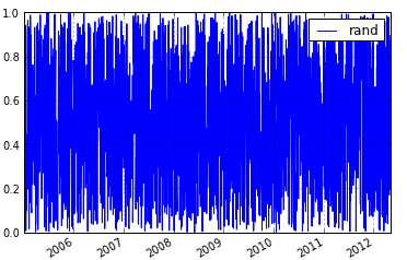
In [11]: %mdf_plot 2005-01-01 T rand
Nodes can be defined interactively either by writing new functions or simply using the nodetype method syntax (nodetype_method_syntax) to build up series of operation quickly
In [12]: %mdf_plot 2005-01-01 T rand.cumprodnode() rand.nansumnode()
This could also be written as
In [13]: a = rand.cumprodnode()

In [14]: b = rand.nansumnode()

In [15]: %mdf_plot 2005-01-01 T a b
In addition to these functions there is also %mdf_dfs which returns a list of
dataframes (one for each node) and %mdf_wp which returns a widepanel constructed
from dataframes for each node. These can be useful when evaluating multiple nodes
at the same time but when you don’t want the results to get merged into a single
dataframe.
Working with Data
Most often data is loaded as a pandas DataFrame, Series or WidePanel. To use those effectively in mdf we normally define a node that is the ‘current’ row or item from that dataset. As time advances that node updates to reveal the data from the underlying structure.
The datanode() function can be used to construct such a node from
any DataFrame, WidePanel or series that is indexed by date.
The following example shows how to access data in a pandas DataFrame:
    from mdf import datanode
    import pandas as pa

# load some data
df = pa.DataFrame.from_csv("data_file.csv")

# create a node whose value is the row from the dataframe for 'now'
df_node = datanode("x", df)
This df_node node is like any other mdf node
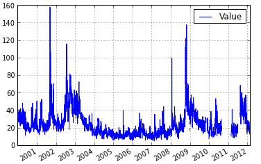
In [18]: %mdf_plot 2000-01-01 T df_node
Applying Functions
Usually when writing code using mdf new nodes are written whenever a value derived from other nodes is required
@evalnode
def df_node_sq():
    return math.pow(df_node(), 2)
For trivial functions such as the one above it can be inconvenient to have to write these for each desired node.
The applynode() function can be used to create new nodes that
apply a function to other nodes. The above example can be re-written as follows:
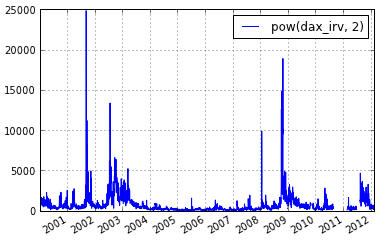
In [19]: df_node_sq = applynode(math.pow, df_node, 2)

In [20]: %mdf_plot 2000-01-01 T df_node_sq
Accessing the Context and Shifting
When you want to evaluate a node with another node set to a specific value or overriden you use a shifted context (see Shifted Contexts).
You can get and set the current ambient context using the %mdf_ctx magic function.
This allows you to get the current context, create a shifted context and then set
that shifted context as the current context.
In [21]: ctx = %mdf_ctx

In [22]: x = varnode(default=1)

In [23]: shifted_ctx = ctx.shift({x : 2})

In [24]: %mdf_ctx shifted_ctx
Out[24]: <ctx 1: 2012-05-03 [x=2] at 123373200>

In [25]: x()
Out[25]: 2
The functions %mdf_df, %mdf_plot and %mdf_xl also take an optional set of
shifts. This makes it easy to get results from a shift without having the get, shift
and set the current context.
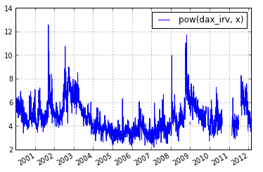
In [26]: df_node_pow = applynode(math.pow, df_node, x)

In [27]: %mdf_plot 2000-01-01 T df_node_pow [x=0.5]
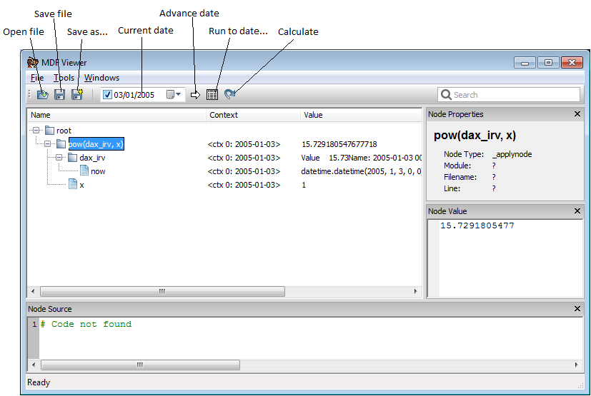
Using the MDF Viewer
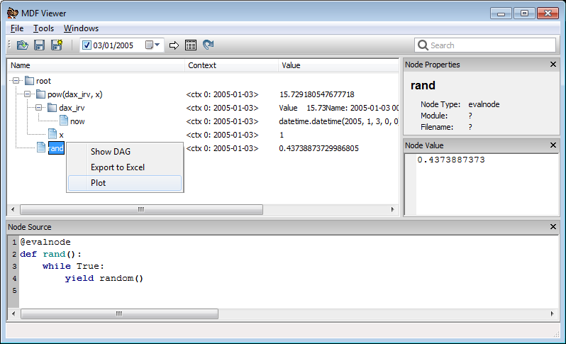
The mdf viewer can be used explore the dependencies between nodes and plot or export values over time.
The mdf viewer can be opened from ipython with the magic command %mdf_show.
In [28]: %mdf_show df_node_pow
More nodes can be added to the open viewer using the same command.
In [29]: %mdf_show rand
To plot or export nodes select the nodes you want (use Shift or Ctrl to select multiple
nodes) and then right click and select plot from the context menu. The same context
menu may be used to export values to Excel or to render a graphical representation
of the graph (requires Graphviz to be installed).
Once the viewer is open you can select one or more nodes and then use the magic command
%mdf_selected to get your current selection in your IPython session
In [29]: %mdf_selected
Out[29]:
[(<ctx 0: 2005-02-11 at 115387248>,
  <<type 'mdf.nodes.MDFEvalNode'> [name=rand] at 0x30fee48>)]
This returns a list of contexts and node objects that correspond to what is selected in the viewer.
The magic functions %mdf_plot, %mdf_df and %mdf_xl can also be used to
plot or get results for the currently selected nodes. To use the currently
selected nodes don’t specify any nodes at all on the command line.
%mdf_plot 2005-01-01 T